Margaret Maynard-Reid
Imports
 ## YOUR CODE HERE ##
%matplotlib inline
The Dataset
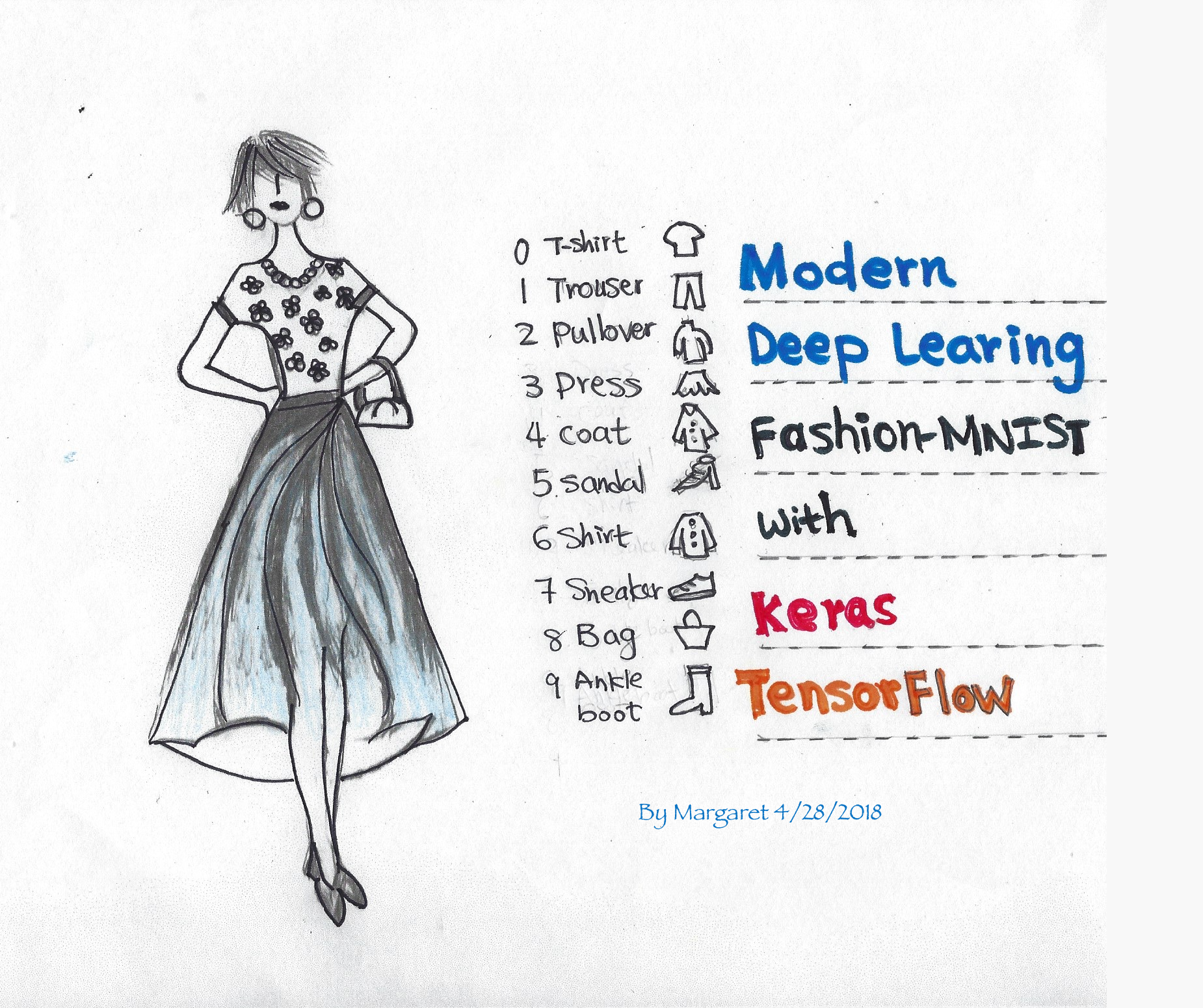
Why Fashion-MNIST?
- MNIST is too easy
- MNIST is overused
- MNIST can not represent modern Computer Vision tasks
Read more about the Fashion-MINST dataset in this paper here (Fashion-MNIST: a Novel Image Dataset for Benchmarking Machine Learning Algorithms)
The fashion_mnist data: 60,000 train and 10,000 test data with 10 categories. Each gray-scale image is 28x28.
Label Description
0 T-shirt/top
1 Trouser
2 Pullover
3 Dress
4 Coat
5 Sandal
6 Shirt
7 Sneaker
8 Bag
9 Ankle boot
Loading data and visualisation
## YOUR CODE HERE ##
# Define the text labels
fashion_mnist_labels = ["T-shirt/top",  # index 0
                        "Trouser",      # index 1
                        "Pullover",     # index 2
                        "Dress",        # index 3
                        "Coat",         # index 4
                        "Sandal",       # index 5
                        "Shirt",        # index 6
                        "Sneaker",      # index 7
                        "Bag",          # index 8
                        "Ankle boot"]   # index 9

# Show first 25 images from the training dataset

plt.figure(figsize=(10,10))
for i in range(25):
    plt.subplot(5, 5, i+1)
    plt.xticks([])
    plt.yticks([])
    plt.imshow(train_images[i], cmap=plt.cm.brg)
    plt.xlabel(fashion_mnist_labels[train_labels[i]])
plt.show()
Data normalization
Normalize the data dimensions so that they are of the same scale. Scale these values to a range of 0 to 1 before feeding them to the neural network model.
# Reshape input data from (28, 28) to (28, 28, 1) as
# mnist.load_data() supplies the MNIST digits with structure (nb_samples, 28, 28)
# The Convolution2D layers in Keras however, are designed to work with 3 dimensions per example
# They have 4-dimensional inputs and outputs. This covers colour images (nb_samples, nb_channels, width, height)

 ## YOUR CODE HERE ##
Split the data into train/validation/test data sets
- Training data - used for training the model
- Validation data - used for tuning the hyperparameters and evaluate the models
- Test data - used to test the model after the model has gone through initial vetting by the validation set.
# Further break training data into train / validation sets
# put 5000 into validation set and keep remaining 55,000 for train)

 ## YOUR CODE HERE ##

# Print training set shape
print("train_images shape:", train_images.shape, "train_labels shape:", train_labels.shape)

# Print the number of training, validation, and test datasets
print(train_images.shape[0], 'train set')
print(x_valid.shape[0], 'validation set')
print(test_images.shape[0], 'test set')
Model Definition
IMG_SIZE = (28, 28, 1)

# Sequential model with the following paramaters:

#Conv2D(filters=64, kernel_size=(2,2), padding='same', activation='relu', input_shape=IMG_SIZE))
#MaxPooling2D(pool_size=(2, 2)))
#Dropout(0.3))

#Conv2D(filters=32, kernel_size=(2,2), padding='same', activation='relu'))
#MaxPooling2D(pool_size=(2, 2)))
#Dropout(0.3))

#Flatten())
#Dense(256, activation='relu'))
#Dropout(0.5))
#Dense(10, activation='softmax'))

# Take a look at the model summary

 ## YOUR CODE HERE ##
Compile the model
Configure the learning process with compile() API before training the model. It receives three arguments:
- An optimizer
- A loss function
- A list of metrics
## YOUR CODE HERE ##
Train the model
Now let's train the model with fit() API.
We use the ModelCheckpoint API to save the model after every epoch. Set "save_best_only = True" to save only when the validation accuracy improves.
history = model.fit(train_images,
         train_labels,
         batch_size=64,
         epochs=3,
         validation_data=(x_valid, y_valid))
plt.plot(history.history['accuracy'], label='accuracy')
plt.plot(history.history['val_accuracy'], label='val_accuracy')
plt.xlabel('Epoch')
plt.ylabel('Accuracy')
plt.ylim([0.7, 1])
plt.legend(loc='best')
plt.plot(history.history['loss'], label='loss')
plt.plot(history.history['val_loss'], label='val_loss')
plt.xlabel('Epoch')
plt.ylabel('Loss')
plt.legend(loc='best')
Test Accuracy
# Evaluate the model on test set
 ## YOUR CODE HERE ##
Visualize prediction
Now let's visualize the prediction using the model you just trained. First we get the predictions with the model from the test data. Then we print out 15 images from the test data set, and set the titles with the prediction (and the groud truth label). If the prediction matches the true label, the title will be green; otherwise it's displayed in red.
y_hat = model.predict(test_images)

# Plot a random sample of 10 test images, their predicted labels and ground truth
figure = plt.figure(figsize=(20, 8))
for i, index in enumerate(np.random.choice(test_images.shape[0], size=15, replace=False)):
    ax = figure.add_subplot(3, 5, i + 1, xticks=[], yticks=[])
    # Display each image
    ax.imshow(np.squeeze(test_images[index]))
    predict_index = np.argmax(y_hat[index])
    true_index = np.argmax(test_labels[index])
    # Set the title for each image
    ax.set_title("{} ({})".format(fashion_mnist_labels[predict_index],
                                  fashion_mnist_labels[true_index]),
                                  color=("green" if predict_index == true_index else "red"))
Congragulations!
You have successfully trained a CNN to classify fashion-MNIST.